This report and accompanying digital interactive tool are based on a nationally representative Pew Research Center survey of 34,897 U.S. adults, conducted October 15-November 8, 2018, on both the Center’s American Trends Panel (ATP) and Ipsos’s KnowledgePanel. The first part of the report presents the survey results at the national level. The second and third parts of the report, as well as the interactive tool, analyze and present survey results at the local level, using CBSAs – or core-based statistical areas – as the main unit of analysis. (See more on what a CBSA is below.) This report was made possible by The Pew Charitable Trusts, the Center’s primary funder, which received support from the Google News Initiative.
The ATP and KnowledgePanel are national probability-based online panels of U.S. adults. Panelists participate via self-administered web surveys. On both the ATP and KnowledgePanel, panelists who do not have internet access are provided with an internet connection and device that can be used to take surveys. Interviews are conducted in both English and Spanish. The ATP is managed by Ipsos.
All active ATP panel members were invited to participate in this survey. All members of the KnowledgePanel living in the 53 most populous CBSAs were invited to participate, while those in less populous CBSAs were sampled at a lower rate. Of the 34,897 respondents in total, 10,654 came from the ATP and 24,243 came from the KnowledgePanel.
The ATP was created in 2014, with the first cohort of panelists invited to join the panel at the end of a large, national, landline and cellphone random-digit-dial survey that was conducted in both English and Spanish. Two additional recruitments were conducted using the same method in 2015 and 2017, respectively. Across these three surveys, a total of 19,718 adults were invited to join the ATP, of which 9,942 agreed to participate.
In August 2018, the ATP switched from telephone to address-based recruitment. Invitations were sent to a random, address-based sample (ABS) of households selected from the U.S. Postal Service’s Delivery Sequence File. In each household, the adult with the next birthday was asked to go online to complete a survey, at the end of which they were invited to join the panel. For a random half-sample of invitations, households without internet access were instructed to return a postcard. These households were contacted by telephone and sent a tablet if they agreed to participate.
KnowledgePanel uses a combination of random-digit dialing (RDD) and address-based sampling (ABS) methodologies to recruit panel members (in 2009 KnowledgePanel switched its sampling methodology for recruiting members from RDD to ABS).
KnowledgePanel continually recruits new panel members throughout the year to offset panel attrition as people leave the panel.
 Weighting
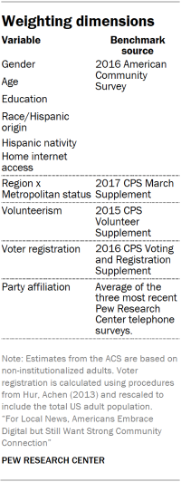
The data were weighted in a multistep process that begins with a base weight incorporating the respondents’ original survey selection probability and the fact that in 2014 and 2017 some ATP respondents were subsampled for invitation to the panel. The next step in the weighting uses an iterative technique that aligns the sample to population benchmarks on the dimensions listed in the accompanying table.
A total of 34,897 panelists responded out of 62,757 who were sampled, for a response rate of 56%. The cumulative response rate accounting for nonresponse to the recruitment surveys and attrition is 1.8%. The margin of sampling error for the full sample of 34,897 respondents is plus or minus 0.8 percentage points.
Sampling errors and statistical-significance tests take into account the effect of weighting. In addition to sampling error, one should bear in mind that question wording and practical difficulties in conducting surveys can introduce error or bias into the findings of opinion polls.
Main source for local news
In an open-ended question, respondents were asked to volunteer the news source they turn to most often for local news. This allowed respondents to write in any news organization or source, not limiting them to specific providers. Researchers grouped these open-ended responses together by brand. For example, responses such as “Chicago Tribune,” “chicago trib” and “chicagotribune.com” were all grouped together under Chicago Tribune.
Researchers took several steps to analyze more than 16,000 individual responses in 31 CBSAs with enough respondents to permit their individual analysis (see list below). Results were analyzed separately for each individual CBSA. The local news sources shown in the report and in the interactive are those that were named by multiple people and by at least 2% of the weighted sample in a CBSA. Local news sources not meeting this threshold in an individual CBSA were coded as “Other.”
Volunteered local news sources based outside of the respondent’s CBSA are shown when they meet the reporting threshold; otherwise they are grouped into “Other.” For example, in Boston, 3% named WMUR, a local television station that serves the neighboring Manchester, New Hampshire, area. Given Manchester’s proximity to Boston, WMUR is the main source of local news for a small portion of Boston residents and is therefore listed as a local news source of Boston-area residents in the interactive. Daily newspapers of large cities (e.g. The New York Times, Los Angeles Times) were coded as local news sources.
Responses that included incomplete or misspelled source names were categorized as the outlets they refer to if the intended source was reasonably clear (e.g., “Sun-Times” named by a Chicago resident was categorized under “Chicago Sun-Times”; “Times” was not). If respondents named a TV network affiliate (e.g. “ABC station”) without specifying a call sign, those responses were grouped under the call sign for the corresponding network affiliate that serves that CBSA. In cases when two channels with the same network affiliate were named by respondents in the same CBSA, the responses were grouped separately as long as respondents explicitly identified the channel in some way (e.g., KESQ); any responses that did not include a specific channel (e.g., respondents said “ABC station”) were listed separately (e.g., “ABC – Unspecified”) and not grouped into either channel. Responses that named TV stations and radio stations with the same call sign and the same ownership/affiliation were grouped together.14 If responses named a call sign that belongs to both a TV and radio station under a different ownership/affiliation, the responses are individually labeled as TV or radio; if responses did not indicate whether they referred to the TV or the radio station they were labeled as “unspecified.”
Results for the 31 CBSAs coded in the interactive and the report were individually produced and reviewed by three researchers.
There were some limited cases where respondents did not name a local news source as their main source for local news. Responses that name a national source are grouped into “National news source.” In addition, respondents who did not provide a response, or gave a response indicating they do not have or do not know their main source (e.g., “N/A,” “None,” “DK”), are listed separately as “None/Refused.”
For local main source results for the 31 CBSAs, visit the accompanying digital interactive tool.
CBSAs included in main source analysis
Below is a list of the 31 CBSAs for which the main source open end was analyzed.
| 1. Atlanta-Sandy Springs-Roswell, GA
2. Baltimore-Columbia-Towson, MD 3. Boston-Cambridge-Newton, MA-NH 4. Chicago-Naperville-Elgin, IL-IN-WI 5. Cincinnati, OH-KY-IN 6. Cleveland-Elyria, OH 7. Columbus, OH 8. Dallas-Fort Worth-Arlington, TX 9. Denver-Aurora-Lakewood, CO 10. Detroit-Warren-Dearborn, MI 11. Houston-The Woodlands-Sugar Land, TX 12. Indianapolis-Carmel-Anderson, IN 13. Kansas City, MO-KS 14. Los Angeles-Long Beach-Anaheim, CA 15. Miami-Fort Lauderdale-West Palm Beach, FL 16. Milwaukee-Waukesha-West Allis, WI |
17. Minneapolis-St. Paul-Bloomington, MN-WI
18. New York-Newark-Jersey City, NY-NJ-PA 19. Orlando-Kissimmee-Sanford, FL 20. Philadelphia-Camden-Wilmington, PA-NJ-DE-MD 21. Phoenix-Mesa-Scottsdale, AZ 22. Pittsburgh, PA 23. Portland-Vancouver-Hillsboro,OR-WA 24. Riverside-San Bernardino-Ontario, CA 25. St. Louis, MO-IL 26. San Antonio-New Braunfels, TX 27. San Diego-Carlsbad, CA 28. San Francisco-Oakland-Hayward, CA 29. Seattle-Tacoma-Bellevue, WA 30. Tampa-St. Petersburg-Clearwater, FL 31.Washington-Arlington-Alexandria, DC-VA-MD-WV |
Local area analysis and interactive tool
Part Two of the report is a closer look at four individual core-based statistical areas (CBSAs): San Antonio-New Braunfels, TX; Minneapolis-St. Paul-Bloomington, MN-WI; Riverside-San Bernardino-Ontario, CA; and Cincinnati, OH-KY-IN. The accompanying digital interactive tool presents results for 99 of the 933 CBSAs in the United States (see below for CBSA description). The estimates for these individual CBSAs were produced using a method known as multilevel regression and poststratification (MRP), a statistical method designed to compute more precise estimates for small subgroups than is possible with conventional survey analysis techniques such as those used for the main survey analysis in this report. The remaining 833 CBSAs were organized into six groups consisting of CBSAs with similar community characteristics, and estimates shown in the digital interactive tool correspond to these groupings. (One CBSA – Vineyard Haven, MA – was not included because the Census API did not consistently return data for it.) For example, when a user searches for data on Topeka, Kansas, the interactive tool will show results for the group Topeka belongs to, which also includes 219 other local areas. This is also explained in more detail below.
It is not possible to use MRP to produce more precise estimates for the main sources of local news in individual CBSAs. This is because each CBSA has its own, unique set of local news sources, while MRP would require that the response options be the same for every CBSA. Instead, the main source estimates shown in the online interactive tool and in the report are estimated using the same survey weights and methods as the national estimates in Part One of the report. As a result, they are shown only for the 31 CBSAs with a sufficiently large number of respondents.
What are CBSAs?
CBSAs – or core-based statistical areas – are geographic areas defined by the U.S. federal government as consisting of at least one urban core of 10,000 people or more, plus adjacent counties that are socio-economically tied to the urban center.
There are two types of CBSAs: metropolitan statistical areas and micropolitan statistical areas. A metropolitan statistical area must have at least one urban core with a population of 50,000 or more inhabitants. A micropolitan statistical area must have at least one urban core with a population of at least 10,000 and less than 50,000 people. In total, there are 933 CBSAs in the 50 states and the District of Columbia, comprised of 1,825 counties. About 94% of Americans live in one of these CBSAs. According to the U.S. Census Bureau’s 2016 Population Estimates, the median CBSA contains about 74,000 residents. Nationally, population size is unevenly distributed, with only 40 CBSAs accounting for about half of the total U.S. population. With a population of over 20 million people, New York-Newark-Jersey City, NY-NY-PA is the largest CBSA in the country. Vernon, TX, Craig, CO, and Lamesa, TX, each with a population of about 13,000, are the smallest CBSAs in the country. (One CBSA – Vineyard Haven, MA – was not included because the Census API did not consistently return data for it.)
There are also 1,317 counties that do not belong to any CBSA because they do not meet the inclusion criteria. Containing 6% of the population, these counties are more rural and sparsely populated than counties belonging to CBSAs.
When looking at local news, counties are sometimes grouped in designated market areas (DMAs), commonly referred to as media markets. A DMA is a group of counties that are all primarily covered by the same set of local network television stations. This means that people who live in the same DMA all get the same local news broadcasts, even though they may live in different cities or counties. There are 210 DMAs across the continental United States, Hawaii, and parts of Alaska, according to Nielsen, versus 933 CBSAs. This means that many DMAs cover multiple CBSAs.
For this analysis, researchers chose CBSAs as the unit of analysis because unlike DMAs, whose boundaries are defined by the range of television broadcasts, CBSAs are designed to be groups of counties that share a level of social and economic integration. When it comes to local news, two CBSAs that belong to the same DMA may not be equally well served by their local stations. Additionally, there is a wealth of supplementary data about CBSAs (or that can be aggregated to the CBSA level) that can be obtained from the U.S. Census Bureau and other sources. The survey sample of about 35,000 respondents offers a unique opportunity to study these kinds of community dynamics and delve into people’s local news habits and attitudes beyond their TV market.
On first reference in the report and the interactive, CBSAs are referred to by their full name as used by the Census Bureau, such as “Scranton–Wilkes-Barre–Hazleton, PA.” Subsequent references refer to the main population center. In this example, the report uses “Scranton, PA” or the “Scranton area” in secondary references.
Multilevel regression and poststratification
To maximize the number of CBSAs that could be reported individually in the online interactive tool, researchers employed a technique called multilevel regression and poststratification (MRP). MRP is a statistical method designed to allow more precise survey estimates, that is, estimates with a smaller margin of error, for subgroups with sample sizes that are too small to analyze with conventional methods.15
For this study, MRP involved first fitting a multilevel regression model to the survey data with the outcome variable of interest as the dependent variable, and a combination of respondent demographics and aggregate CBSA characteristics drawn from external sources (e.g., population size or median household income) as independent variables. This model is then used to predict the value of the dependent variable for all noninstitutionalized adults in the 2016 American Community Survey 1-Year Public Use Microdata Sample (PUMS). Finally, estimates are calculated using the average of the predicted values for the ACS respondents in each CBSA.
Multilevel regression model specification
The first step in computing survey estimates with MRP involved fitting multilevel regression models for each dependent variable.16 The models were fit using the Bayesian regression modeling package brms for the R statistical computing platform.17 Logistic regression was used for variables with only two response options. Categorical variables with more than two response options were modeled using multinomial logistic regression, while variables with ordered response options (e.g., Very, Somewhat, A little, Not at all) were modeled using cumulative logistic regression.
 All of the regression models used the same basic specification. It assumed variable intercepts with crossed random effects for CBSA and state, and respondent-level main effects for age, sex, race and Hispanic ethnicity, home internet access, and census division.18
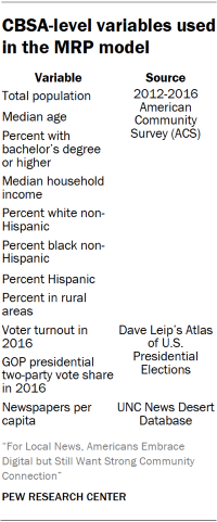
CBSA-level variables were obtained from external data sources and appended to the survey data, meaning that respondents who came from the same CBSA all had the same values for the appended variables. These variables are listed in the accompanying table along with their respective sources. Before being appended to the survey data, CBSA-level variables with skewed distributions were transformed to be more symmetrical. For computational reasons all CBSA-level variables were standardized and mean-centered.
These models were fit using a Bayesian framework, which means that it is necessary to specify a prior distribution for each parameter in the model. These models used uniform or “flat” priors for the intercepts and regression coefficients. The prior distributions for the state and CBSA random effects were set to the default values for the brms package, specifically a t-distribution with three degrees of freedom, a mean of zero and a standard deviation of 10.
Because not all the variables used in the survey weighting are asked on the American Community Survey (ACS), the main survey weights were used in the regression to minimize inconsistencies between the MRP estimates and the weighted survey estimates used throughout the report. With the brms package, this is done by making each case’s contribution to the log likelihood proportional its weighted value.
Poststratification
Computing MRP estimates for an individual CBSA requires knowing what share of its adult population belongs to every possible combination of characteristics defined by the independent variables in the model, specifically age, sex, race/ethnicity, home internet access, state and census division. These figures were calculated using the 2016 American Community Survey 1-Year Public Use Microdata Sample (PUMS).
For privacy reasons, the Census Bureau does not release CBSA as part of its ACS PUMS files. Instead, the smallest geographic unit available for respondents is their public use microdata area (PUMA). PUMAs are geographically contiguous groups of census tracts and counties containing at least 100,000 people. Of the 2,351 PUMAs in the United States, 1,872 (about 80%) are entirely contained within a single CBSA, or have portions that do not belong to any CBSA. The remaining 479 PUMAs have portions falling into two or more CBSAs. This means that for ACS respondents from these crossover PUMAs, it is not possible to know with certainty the CBSA in which they truly reside.
To address the mismatch between PUMA and CBSA, researchers applied the following procedure for each CBSA. First, the ACS data were filtered to cases from those PUMAs that are either partially or completely contained within the CBSA. The weights for those cases were then multiplied by the proportion of the PUMA’s population that lives in that CBSA according to figures from the 2010 decennial census.19 This approach assumes that individuals who live in the same PUMA but different CBSAs do not differ substantially with respect to their demographic distributions. Researchers validated this assumption by comparing each CBSA’s demographic distributions calculated using these modified PUMS weights to pre-tabulated Census estimates based on the complete, nonpublic ACS dataset and found the differences to be negligible.
Next, a poststratification frame for the CBSA was created by assigning every ACS respondent to a cell based on the full cross-classification of sex, age, race/ethnicity, home internet access, state and census division. The CBSA-level variables used in the model were then appended, and the number of adults belonging to each cell was calculated as the sum of the weights for each ACS respondent in that cell.
In the last step, a regression model was used to predict the mean values of the dependent variable for every cell in the CBSA. For a given dependent variable, the overall estimate for the entire CBSA is then the average of the cell-means weighted by their size. This process is repeated for every dependent variable and every CBSA.
The level of uncertainty for every estimate was computed by summarizing 2,000 draws from each regression model’s posterior predictive distribution. The point estimates discussed are the mean values over the posterior distribution for each estimate. The “modeled margin of error” for each estimate is half the width of a 95% Bayesian credibility interval. Although they have different philosophical interpretations, this quantity was intentionally chosen due to its similarity to the more familiar “margin of sampling error” commonly reported by pollsters, that is, half of the width of a 95% frequentist confidence interval.
Although MRP made it possible to report individual estimates for many more CBSAs than would have been possible using standard methods, there were still many CBSAs for which sufficiently precise estimates were not possible. The 99 CBSAs reported individually were those for which all the MRP estimates to be included in either the report or the digital interactive tool had a modeled margin of error less than 12 percentage points. This threshold was chosen to balance the competing interests of reporting on as large and diverse a set of communities as possible while ensuring that all the estimates shown met at least some minimum standard for precision.
It is important to note that a margin of error of 12 percentage points is not typical, but rather the maximum for any single estimate out of a total of 147 separate estimates calculated across 51 different variables. For the 99 CBSAs, most estimates are much more precise, with an average modeled margin of error of plus or minus 4.2 percentage points. The CBSA with the least precise estimates was Salem, Oregon, where the average came to plus or minus 6.2 points, and even in this case about a third of the estimates have margins of error under 4 points.
CBSAs individually shown in the online interactive tool
Below is a list of the 99 CBSAs for which results are estimated using MRP, and which are shown individually in the interactive. Collectively they cover approximately 66% of the total population in the 50 states and the District of Columbia.
|
1. Akron, OH 2. Albany-Schenectady-Troy, NY 3. Albuquerque, NM 4. Allentown-Bethlehem-Easton, PA-NJ 5. Atlanta-Sandy Springs-Roswell, GA 6. Austin-Round Rock, TX 7. Bakersfield, CA 8. Baltimore-Columbia-Towson, MD 9. Baton Rouge, LA 10. Birmingham-Hoover, AL 11. Boise City, ID 12. Boston-Cambridge-Newton, MA-NH 13. Bridgeport-Stamford-Norwalk, CT 14. Buffalo-Cheektowaga-Niagara Falls, NY 15. Cape Coral-Fort Myers, FL 16. Charlotte-Concord-Gastonia, NC-SC 17. Chicago-Naperville-Elgin, IL-IN-WI 18. Cincinnati, OH-KY-IN 19. Cleveland-Elyria, OH 20. Columbia, SC 21. Columbus, OH 22. Corpus Christi, TX 23. Dallas-Fort Worth-Arlington, TX 24. Dayton, OH 25. Deltona-Daytona Beach-Ormond Beach, FL 26. Denver-Aurora-Lakewood, CO 27. Des Moines-West Des Moines, IA 28. Detroit-Warren-Dearborn, MI 29. El Paso, TX 30. Fayetteville-Springdale-Rogers, AR-MO 31. Fresno, CA 32. Grand Rapids-Wyoming, MI 33. Greensboro-High Point, NC 34. Greenville-Anderson-Mauldin, SC 35. Harrisburg-Carlisle, PA 36. Hartford-West Hartford-East Hartford, CT 37. Houston-The Woodlands-Sugar Land, TX 38. Indianapolis-Carmel-Anderson, IN 39. Jacksonville, FL 40. Kansas City, MO-KS 41. Knoxville, TN 42. Lakeland-Winter Haven, FL 43. Lancaster, PA 44. Las Vegas-Henderson-Paradise, NV 45. Lexington-Fayette, KY 46. Los Angeles-Long Beach-Anaheim, CA 47. Louisville/Jefferson County, KY-IN 48. Madison, WI 49. McAllen-Edinburg-Mission, TX 50. Memphis, TN-MS-AR |
51. Miami-Fort Lauderdale-West Palm Beach, FL 52. Milwaukee-Waukesha-West Allis, WI 53. Minneapolis-St. Paul-Bloomington, MN-WI 54. Modesto, CA 55. Myrtle Beach-Conway-North Myrtle Beach, SC-NC 56. Nashville-Davidson–Murfreesboro–Franklin, TN 57. New Haven-Milford, CT 58. New Orleans-Metairie, LA 59. New York-Newark-Jersey City, NY-NJ-PA 60. North Port-Sarasota-Bradenton, FL 61. Ogden-Clearfield, UT 62. Oklahoma City, OK 63. Omaha-Council Bluffs, NE-IA 64. Orlando-Kissimmee-Sanford, FL 65. Philadelphia-Camden-Wilmington, PA-NJ-DE-MD 66. Phoenix-Mesa-Scottsdale, AZ 67. Pittsburgh, PA 68. Portland-South Portland, ME 69. Portland-Vancouver-Hillsboro, OR-WA 70. Providence-Warwick, RI-MA 71. Provo-Orem, UT 72. Raleigh, NC 73. Richmond, VA 74. Riverside-San Bernardino-Ontario, CA 75. Rochester, NY 76. Sacramento–Roseville–Arden-Arcade, CA 77. Salem, OR 78. Salt Lake City, UT 79. San Antonio-New Braunfels, TX 80. San Diego-Carlsbad, CA 81. San Francisco-Oakland-Hayward, CA 82. San Jose-Sunnyvale-Santa Clara, CA 83. Scranton–Wilkes-Barre–Hazleton, PA 84. Seattle-Tacoma-Bellevue, WA 85. Spokane-Spokane Valley, WA 86. Springfield, MA 87. St. Louis, MO-IL 88. Stockton-Lodi, CA 89. Tampa-St. Petersburg-Clearwater, FL 90. Toledo, OH 91. Tucson, AZ 92. Tulsa, OK 93. Urban Honolulu, HI 94. Virginia Beach-Norfolk-Newport News, VA-NC 95. Visalia-Porterville, CA 96. Washington-Arlington-Alexandria, DC-VA-MD-WV 97. Wichita, KS 98. Worcester, MA-CT 99. Youngstown-Warren-Boardman, OH-PA |
The digital interactive: How Pew Research Center used clustering to provide estimates for groups of CBSAs
Even with the large sample size and MRP modeling, there are 833 CBSAs for which individual estimates could not be computed with sufficient precision. To allow members of the public who may be from those areas to still get a sense of local news habits in their local area, CBSAs with similar characteristics were grouped together. Estimates shown are for these groups of similar CBSAs rather than the individual CBSAs. The clustered estimates are also calculated using MRP. These groupings were formed using unweighted hierarchical clustering, which organized CBSAs using a variety of external data. Selecting the final clusters was an iterative process that involved experimentation with several clustering techniques and evaluating dozens of different combinations of CBSA characteristics taken from external data sources.
External data collection and variable selection for the clustering
The Center used a variety of CBSA-level variables, such as racial diversity, age, income and broadband penetration to create the different clusters.
About 80 different CBSA-level variables were collected for this analysis from the 2012-2016 American Community Survey (ACS). Also collected were data on voter turnout using 2016 voting data from Dave Leip’s Atlas of U.S. Presidential Elections and newspaper data from “The Expanding News Desert Database” by the University of North Carolina School of Media and Journalism’s Center for Innovation and Sustainability in Local Media. All ACS variables were downloaded via the Census API at the CBSA level. Newspaper data were provided at both the county and CBSA level and analyzed at the CBSA level. Voting variables (2016 voter turnout and the 2016 GOP presidential two-party vote share) were calculated by combining the number of votes in each county to get the number of raw votes per CBSA. Because Alaska does not report election results at the county level, the same statewide results were assigned to each of the four CBSAs in that state. Broadband access data relied on the 2013-2017 ACS because that was the first five-year dataset that included responses from all CBSAs for the broadband question used here.
Researchers first took steps to pare down the number of variables to be considered for use in the clustering. First, variables that correlated strongly with others were removed. For example, the households with internet variable had a high correlation (above 0.85) with the households with computers variable, so the households with computers variable was removed. In addition, researchers tried a variety of combinations of variables and removed those that consistently did not influence the results. Finally, population was transformed into quartiles to reduce the disproportionate effect of its highly skewed distribution. After these steps, 13 variables were used for the clustering, coming from the following sources:
U.S. Census Bureau’s 2012-2016 American Community Survey
- Population quartile
- Black (not Hispanic) percent of population
- Hispanic (of any race) percent of population
- White (not Hispanic) percent of population
- Median age
- Percent of population with at least a bachelor’s degree
- Percent of population in rural areas
- Median household annual income
- Percent of population under the poverty line
U.S. Census Bureau’s 2013-2017 American Community Survey
- Percent of households with broadband access via DSL, cable or fiber optic
Dave Leip’s Atlas of U.S. Presidential Elections
- Voter turnout in 2016, calculated by dividing the number of people that voted in the 2016 presidential election by the number of people over 18 (from the 2016 ACS 5-year file)
- GOP presidential two-party vote share in 2016, calculated by dividing the number of votes Trump received by the number of votes Trump and Clinton received
UNC’s School of Media and Journalism’s Center for Innovation and Sustainability in Local Media News Desert Database:
- Newspapers per capita
Unweighted hierarchical clustering
Several clustering techniques were tested using these data, including k-means clustering, hierarchical clustering and weighted clustering. Because the number of clusters must be selected in advance, final models were tested with between seven to 20 clusters. Models were evaluated according to whether or not the CBSA groupings made intuitive sense not just quantitatively but also substantively and qualitatively. Solutions that resulted in individual clusters that were disproportionately too large or too small to be analytically valuable were avoided. There were 833 CBSAs clustered this way; the 99 CBSAs for which individual estimates are reported were not included in the clustering analysis.
Ultimately, researchers settled on an unweighted hierarchical clustering model with nine clusters. Clusters with a sample size too small to analyze were combined with other similar clusters, resulting in six distinct clusters. Although the assessment necessarily involved a degree of subjectivity, this clustering solution was found to yield a relatively small set number of well-sized groups whose composition also made intuitive sense from a substantive perspective.
Analysis of local area characteristics
Many CBSAs share common characteristics, such as size, density and ethnic makeup of the population, that may impact how residents get news about their local area. This report examines how people’s local news habits and attitudes differ based on certain community characteristics such as age, household income, racial and ethnic diversity, broadband internet access and voter turnout. Unlike in the metro area analysis, this community analysis examines survey results across 932 CBSAs, using national survey weighting instead of the individual CBSA MRP estimates explained above.20 The variables used and the steps taken to analyze them are below.
Data sources used in the community analysis
The publicly available data sources used and the community-level variables pulled from each include:
U.S. Census Bureau’s 2012-2016 American Community Survey
- Black (not Hispanic) percent of population
- Hispanic (of any race) percent of population
- White (not Hispanic) percent of population
- Median age
- Median annual household income
U.S. Census Bureau’s 2013-2017 American Community Survey
- Percent of households with broadband access via DSL, cable or fiber optic
Dave Leip’s Atlas of U.S. Presidential Elections
- Voter turnout in 2016, calculated by dividing the number of people that voted in the 2016 presidential election by the number of people over 18 (from the 2016 ACS 5-year file)
Defining the lower, medium and higher comparative groups
All of the publicly available data used in this analysis were collected at either the CBSA or county level of geography. When the external data were available at the county level only, the data were grouped into CBSAs using the Census Bureau’s August 2017 CBSA delineation file (all ACS data were collected at the CBSA level, while election data were collected at the county level). For each community-level variable, researchers categorized CBSAs into three comparative groups:
- Lower group – includes CBSAs that rank relatively low in the community-level variable
- Higher group – includes CBSAs that rank relatively high in the community-level variable
- Medium group – includes the remaining CBSAs
To create these three groups, researchers found appropriate cutoff values for the community-level variable so that the lower and higher groups each comprised – in most cases – about 10% of the U.S. population residing in CBSAs.
Defining the lower group
- CBSAs were first sorted by the community-level variable in ascending For example, the percent of the Hispanic population variable was sorted from lowest percentage (i.e., the CBSA with the smallest proportion of Hispanics, at 0.1%) to highest percentage (i.e., the CBSA with the largest proportion of Hispanics, at 99.0%).
- Researchers then determined the cutoff value for the community-level variable by determining the CBSAs containing the 10% of the population with the lowest values for that variable. This was done by moving down the list of CBSAs (sorted by the variable being considered) and summing the population of each CBSA until the sum reaches 10% of the total population residing in CBSAs (excluding those who do not live in a CBSA). The value for the community-level variable for this CBSA is the cutoff value for the lower group.
- All CBSAs with a community-level variable value that is less than or equal to this cutoff value were included in the lower group.
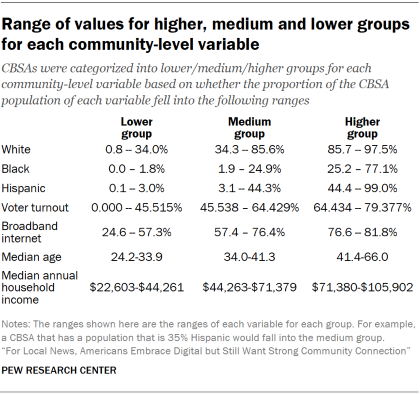 For instance, for the community-level variable measuring the percent of Hispanic population, the cutoff value for the lower group is 3.0% (the minimum value at which the summed population is about 10% of the total population residing in CBSAs). Therefore, the lower group is defined as CBSAs with a Hispanic population that is less than or equal to 3.0%.
Defining the higher group
- CBSAs were first sorted by the community-level variable in descending order (the sort was in ascending order when defining the lower group). For example, the percent of the Hispanic population variable was sorted from highest percentage (i.e., the CBSA with the largest proportion of Hispanics, at 99.0%) to lowest percentage (i.e., the CBSA with the smallest proportion of Hispanics, at 0.1%).
- Researchers then determined the cutoff value for the community-level variable by determining the CBSAs containing the 10% of the population with the highest values for that variable. This was done by moving down the list of CBSAs (sorted by the variable being considered) and summing the population of each CBSA until the sum reaches 10% of the total population residing in CBSAs (excluding those who do not live in a CBSA). The value for the community-level variable for this CBSA is the cutoff value for the higher group.
- All CBSAs with a community-level variable value that is greater than or equal to this cutoff value were included in the higher group.
For the variable measuring the percent of Hispanic population, the cutoff value for the higher group is 44.4% (the minimum value at which the summed population is about 10% of the total population residing in CBSAs). Therefore, the higher group is defined as CBSAs with a Hispanic population that is greater than or equal to 44.4%.
Defining the medium group
CBSAs that did not fall into either the lower or higher group make up the medium group.
For the variable measuring the percent of Hispanic population, the medium group is defined as CBSAs with a Hispanic population that is between 3.1% and 44.3%.
For each community-level variable, each survey respondent was coded as high, medium, or low according to the CBSA in which they lived.
